HP41 13-digit OS Routines. Scratching the surface...[]
HP41 OS 13-digit Math Routines.
Scratching the surface 30 years later.

By Ángel M. Martin.
November 2010
This compilation, revision A.1.2.
Copyright © 2010 Ángel M. Martin
Published under the GNU software license agreement.
Intro[]
The purpose of this mini-paper is to document the usage of some of the 13-digit math routines within the 41 OS – for extended precision in the calculations of functions in the SandMath and the 41Z modules. It’s not a comprehensive description of the routines, nor should it be seen as a complete overview of the 41 Math Rom (system ROM_1), which – I’m glad to say – still holds many secret chestnuts and undocumented treasures.
It’s assumed that the reader is familiar with the “standard|” math routines in the OS, such as [AD2_10], [MP2_10], [LN10], etc. I’ll make no attempt to explain those anything beyond a comparison point with the extended ones. I’m not a computer science engineer; so pls. allow some imprecise rigor or unclear use of terms within the descriptions below – you’ve been warned!
The basics: Nibbles and digits[]
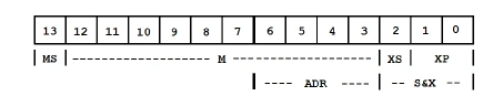
The NUT CPU - a 30-year old classic by today’s standards – uses 7-byte registers as main memory unit. Each byte has two nibbles, each nibble being 4 bits - which makes it a 56-bit CPU, if that means anything these days. Nibbles (or digits) are labeled from right to left as 0 to 13, with nibble 0 holding the LSB. The typical assignment distribution of those fields is as follows:
- nibble 13 holds the sign of the mantissa, called the MS field. A zero denotes positive numbers, and 9 a negative number
- nibbles 12 to 3 hold the mantissa, called the M field and ranging from 0 to 9999999999
- nibble 2 holds the sign of the exponent, called the XS field - with zero positive and 9 negative exp.
- nibbles 1 and 0 (that is: byte 0) hold the exponent, called the XP field ranging from 0 to 99. The combination of nibbles 2 to 0 is also called the S&X field.
Typically a number in the calculator is held in a single register, thus its precision is limited to 10 digits. This was good enough for 1980 standards for calculator design, but as algorithms get more complicated the numerical errors become more significant, rendering the system sub-optimal.
Yet the 41 OS math routines (in ROM1) were written with extended precision in mind. They employ two CPU registers to hold the numbers, extending the actual precision to 13 digits, as follows:
- first register holds MS and the S&X,
- second register holds a 13-digit mantissa.
From this it’s clear that the routines should then operate taking a dual-register definition for each one of the input arguments (one if MONADIC and two if DUAL), and conversely should exit leaving the final result in two registers as well.
But in fact, they’re even better than that.
Considering that the initial input data and the final output result can only have a 10digit form, those routines must also accept 10-digit inputs, and must produce 10-digit outputs. No surprisingly they are indeed designed to accept input on either way, and to output the results in both ways. There’s even a third hybrid form, with one operand in 13-digit form and another in 10-digit form.
This allows intermediate operations to be done with 13-bit precision, which is good enough to achieve a 10-digit accuracy, without rounding errors or loss of resolution.
The important thing to realize is that there is only ONE set of math routines, and not dual sets. The routines always operate on a dual-mode basis, and exit with dual results placed in both 10-digit form [in register C], and 13-digit form [in arithmetic registers A&B].
Different entry points within the routines determine whether it’s using the extended precision or not, just truncating the input values to 10-digit forms. So even the standard [AD2_10] routine produces a 13-digit output in registers A&B, even though most of the time this isn’t taken advantage of and only the result placed in C is used.
So from now on we won’t refer to either 10-digit or 13-digit routines anymore, as there’s only one set – with a choice of manners to use them, depending on the syntax (entry points) and the richness of the data.
This also means the execution time is not longer when the 13-digit forms are used, thus there’s no penalty in using them!
And besides that, to make things even more attractive, the code listings get simplified if the extended precision syntax is used – due to the way the routines have been written, and to the auxiliary routines used to facilitate repeated operations. So typically programs are shorter, saving vital bytes.
Those three reasons are surely good enough to justify the learning curve, won’t you agree? So let’s get to it, shall we…
Entry points and digit forms[]
Clever as they were, the 41 OS programmers followed a nomenclature system to consistently label the different entry points for all routines in a common way, denoting the data form convention to use.
So a dual 10-digit form always uses the “2-10” string in their names, and the dual 13digit form uses “2-13” – whereas the one-of-each hybrid uses “1-10” as descriptor.
All perfectly clear, and very helpful to get your bearings when navigating the MCODE listings.
Let’s first review what we already knew:
- A single 10-digit input for MONADIC functions is expected to be in Register C. This of course notwithstanding additional requirements, like also being in register N (as it’s done with [XFCT100],
- A dual 10-digit input for DUAL functions is expected to be in registers A for the first operand, and register C for the second. Ditto here w.r.t. additional requirements, like also using X/Y (like in [TOPOL] – this one probably the most complex routine in the OS alone!)
And here’s the extension to the knowledge:
- A single 13-digit input for MONADIC functions is expected to be in the arithmetic registers A&B, as per the 13-digit convention explained before. Examples are: [LN13], [SQR13], [EXP13].
- A dual 13-digit input for DUAL functions is expected to be in registers A&B for the first operand, and registers C&M for the second one. The order is especially important for the division routine, of course. Examples are [AD213] , [MP2-13] and [DV2-13]
- A hybrid 10- and 13-digit input for DUAL functions is expected to be in registers A&B for the first operand (13-digit form following the extended convention), and in register C for the second operand (10-digit form following the standard convention). Examples are [AD1-10], [MP1-10] and [DV1-10].
Note that there aren’t entry points for the reverse situation – operand 1 must be the 13-digit form
But wait, there’s more. To further facilitate interoperability within all these routines, there are auxiliary ones that make the chain calculations almost as simple as if we were using an RPN stack. They are:
- [STSCR].- A routine to temporarily store a 13-digit result for later reuse, using scratch registers “Q” &”+” – using a slightly modified convention due to the compromised usage of the “+” register. (Now we know why Q can’t be used in our MCODE so often!)
- [RCSCR].- Its trusty companion, a routine to restore the scratch registers into registers C&M, so their content can be used as second operand by a DUAL function. (It takes care of the subtleties used in [STSCR] to reverse the convention in compatible way).
- [EXSCR].- The third one. A routine to exchange (swap) the contents of registers A&B with the scratch registers. Nothing like the versatility of a swap sometimes!
- [ADDONE], [SUBONE].- handy routines to add/subtract one (written ad-hoc in C) to/from the number held in registers A&B, leaving the result also in A&B. (Guess which native functions used these? Here’s a hint: LNX+1 and E^X-1).
- [PI/2].- There’s never enough number of decimal digits for an irrational number, won’t you say? This routine gives 13 of them, and it’s broadly used all along the Math ROM. Also note that it’s placed in C&M. ready to be used as second operand for addition or multiplication steps.
- [LNC10], [LNC20], [LNC30], [LNC40], [LNC50], etc. As their names imply, routines to input the different values of the decimal log for those relevant values. (I’m a bit fuzzy here as I haven’t really studied them all).
Let’s see some examples of how to use these handy routines, comparing the syntax and code reduction as things get more powerful:
Example 1.- Adding X and Z.[]
No frills here: each input is a 10-digit form so our old-reliable routines do the work – and there’s no additional value in using the 13-digit syntax, as we can’t possibly “guess” the three missing digits!
READ 1(Z)
A=C ALL
READ 3(X)
[AD2-10]
Example 2. Calculate (X+Z)*Y[]
Here’s a good chance to compare the “ standard” vs. the “extended” syntax:
READ 1(Z)	    READ 1(Z)
A=C ALL	    A=C ALL
READ 3(X)	    READ 3(X)
[AD2-10]	    [AD2-10]    - so far so good, but watch:
A=C ALL	    READ 2(Y)   - uh? No need to obliterate A
READ 2(Y)	    [MP1-10]    - an elegant way to finish.
[MP2-10]
Note how we didn’t need to save the intermediate result as 10-digit form into A, as it was ALREADY saved into A&B in 13-digit form. (so saving it would’ve destroyed it). Note also we saved one line whist gaining precision – a great deal.
Example 3. Calculate (X+Z)*(Y+T)[]
C=0 S&X		C=0 S&X	- only way to read the T register
RAMSLCT		RAMSLCT	- select bottom of chip0
READATA		READATA	- get first operand to C
A=C ALL		A=C ALL	- save it in A
READ 2(Y)		READ 2(Y)   - so far so good, but watch:
[AD2-10]		[AD2-10]    - first intermediate result:
N=C			[STSCR]	- saved in scratch
READ 1(Z)		READ 1(Z)
A=C ALL		A=C ALL
READ 3(X)		READ 3(X)
[AD2-10]		[AD1-10]    - second intermediate result
A=C ALL		[RCSCR]	- the trusty companion
C=N			[MP2-13]    - full dual 13-digit glory at last
[MP2-10]
In all fairness there’s not such a code reduction here since the calls to [STSCR] and [RCSCR] required two bytes, whereas using N as scratch register is a single byte each way. Nevertheless the code clarity and enhanced accuracy are always there.
Example 4. Calculate Ln(X)+Y[]
This one also benefits from the extended entry points syntax, as follows:
READ 3(X)		READ 3(X)   - get operand to C
CLRF 5		CLRF 5	- flag the proper logarithm to use
[LN10]		[LN10]	- result in both 10 & 13-digit forms
A=C ALL		READ 2(Y)   - get second operand to C
READ 2(Y)		[AD1-10]    - hybrid multiplication to end
[AD2-10]
Example 5. Calculate SQR(X^2+Y^2) - (a.k.a the module.)[]
READ 3(X)		READ 3(X)   - get first operand to C
A=C ALL		A=C ALL	- duplicate in A
[MP2-10]		[MP2-10]    - square power in both 10/13-digit forms
N=C			[STSCR]	- 13-digit form saved in scratch
READ 2(Y)		READ 2(Y)   - get second operand to C
A=C ALL		A=C ALL	- duplicate in A
[MP2-10]		[MP2-10]    - result in both 10/13-digit forms
A=C ALL		[RCSCR]	- recall first partial result to C&M
C=N			[AD2-13]    - all-13-digit addition to end
[AD2-10]		[SQR13]
[SQR10]
Examples 6 & 7.- Calculate (X^3)+1 and (1/X^2) -1[]
Now without the corresponding comparisons, to expedite the illustration.
a) Adding one	b) Subtracting one

READ 3(X)		READ 3(X)
A=C ALL		A=C ALL
[MP2-10]		[MP2-10]
READ 3(X)		[ON/X13]
[MP1-10]		[SUBONE]
[ADDONE]
Example 8.- A couple of tricks to impress your friends.[]
Calculate 1/X^2, and divide a 10-digit number in N by its value (i.e. the reciprocal to [DV1-10]).
The first part is easy, let’s do it in two different ways::
a) The sub-	    b) the full-
  optimal way	 resolution way

READ 3(X)	    READ 3(X)
[ON/X10]	    [ON/X10]
[MP1-10]	    [STSCR]
		    [RCSCR]
		    [MP2-13]
In the shorter implementation (on the left) we take advantage of the fact that the output from the [1/X] routine is dual, as 13-digit form in A&B and also as a 10-digit form in C. It’s shorter but of course doesn’t utilize the full information available and therefore the longer implementation (on the right) is recommended. If space is at a premium (as it eventually always is), the sub-optimal implementation is still better than a dual 10-digit one – which also takes man extra code line.
The second part is a little trickier. Since there isn’t an entry point to reflect this kind of hybrid scenario, we’ll upgrade the 10-digit value into a “fake”13-digit one in order to use the dual 13-digit division entry point, as follows:
[STSCR]	    - saves A&B in scratch
C<>N	    - puts the 10-digit value to C
A=C ALL	    - puts its sign and X&S in A
B=0 ALL	    - a precaution to clear unused fields
C<>B M	    - puts the 10-digit mantissa in B
[EXSCR]	    - swaps the “fake” upgraded value and the genuine one
[RCSCR]	    - places the fake value into C&M
[DV2-13]	    - performs the division our way
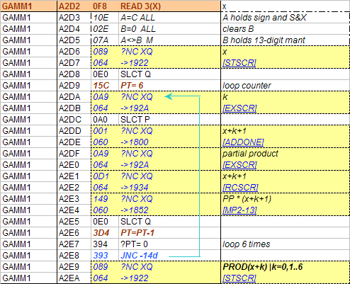
Example 9- Get the gloves off and calculate PROD [X+k], for k=1,2…6[]
Now in a more realistic vein, we’ll approach this one using a more detailed listing description as follows:
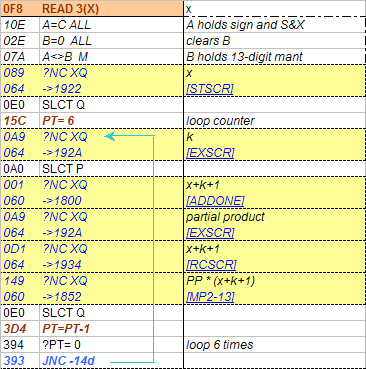
Highlights here are the usage of [EXSCR] and the initial conversion of the input value to a “fake” 13-digit form, so that the same syntax could be used inside of the multiplication loop.
The result of the loop is in 13-digit form, and it’s ready for further chain calculations as need may be.
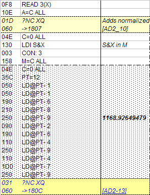
Example 10.- Calculate 2X + 1168,92649479[]
Notice of course that there are 12 digits in all required to define the value to add, therefore we’ll have to use a dual 13-digit form addition. All we need is converting the given number to a proper 13-digit form in order to be able to use all its 12 digits in the adding operation.
This entails not only writing its mantissa in C, but also its sign and S&X into the M register to have a whole-defined value. Also let’s not forget clearing the unused values in either register to avoid sporadic errors, so difficult to troubleshoot.
Example 11.- Pi in the sky.[]
Working with PI has two variants, depending on whether it’s used as first or second operand. Remember that [PI/2] writes a 13-digit version of p into the C&M registers, so it’s ready as a second argument but requires some work it it’s to be used as first:
For instance, to calculate the square root of 2*PI
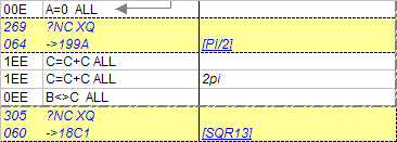
And to divide a 13-digit form number by PI
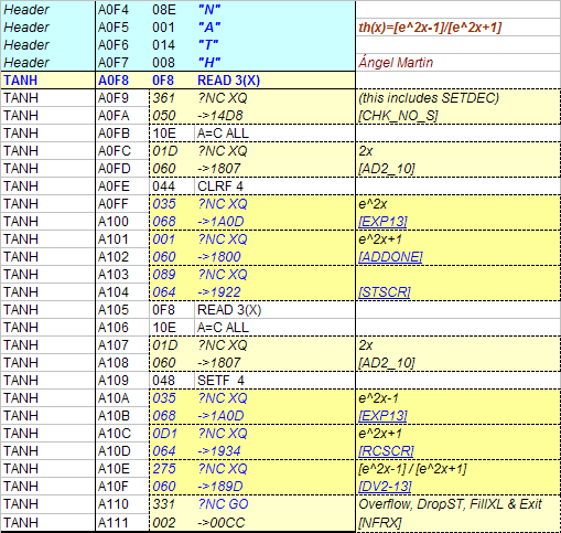
A real-life example: Hyperbolic functions at last.[]
Yes there are many unanswered questions in the universe, but certainly one of them is why, oh why, didn’t HP-MotherGoose provide a decent set of hyperbolic functions in the (otherwise pathetic) MATH-PAC, and worse yet -adding insult to injury- how come that error wasn’t corrected in the Advantage ROM?
For sure we’ll never know, so it’s about time we move on and get on with our lives – whilst correcting this forever and ever.
The first incarnation of these functions came in the AECROM module; I believe programmed by Nelson C. Crowle, a real genius behind such ground-breaking module - but it was also somehow limited to 10-digit precision.
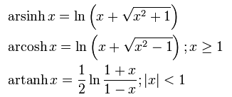
Here they are in all their 13-digit splendor at last.[]
First the inverse functions, using the logarithm and square root routines.
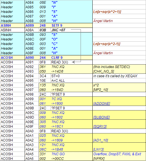
We could’ve used a “fake” 13-digit format for X to have access to [ADDONE] and [SUBONE], but that wouldn’t have added any more precision to the result.
Instead we used the [LN1+X] routine, which internally does the same thing anyway.
And of course we’ll utilize its 13-digit output!
On the other hand, we use the scratch registers to store the partial result Ln(1+x), so that it’ll be fully used as 13-digit value in the final subtraction step.
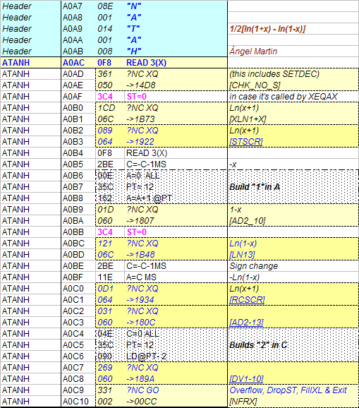
And here are the direct functions, a festival of exponential routines for you:
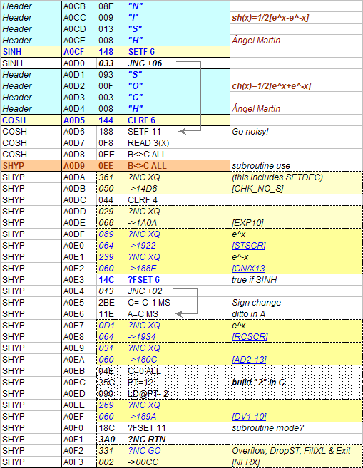
Here the usage of a subroutine and CPU flag 11 is due to the fact that the LogGamma function (elsewhere in the SandMath) requires calculating the hyperbolic sine as intermediate step, otherwise it could have a shorter listing, and without using register B either.
![]()
Note also the common ending in these, suitable to yet further space savings just by using a JNC call to the appropriate section. We have however left it like that for clarity.
Go ahead and set your machine in FIX 9, and bang the keyboard with esoteric inputs until you get blue in the face – do you find rounding errors somewhere? :-) - Hint: use www.wolframalpha.com as reference.
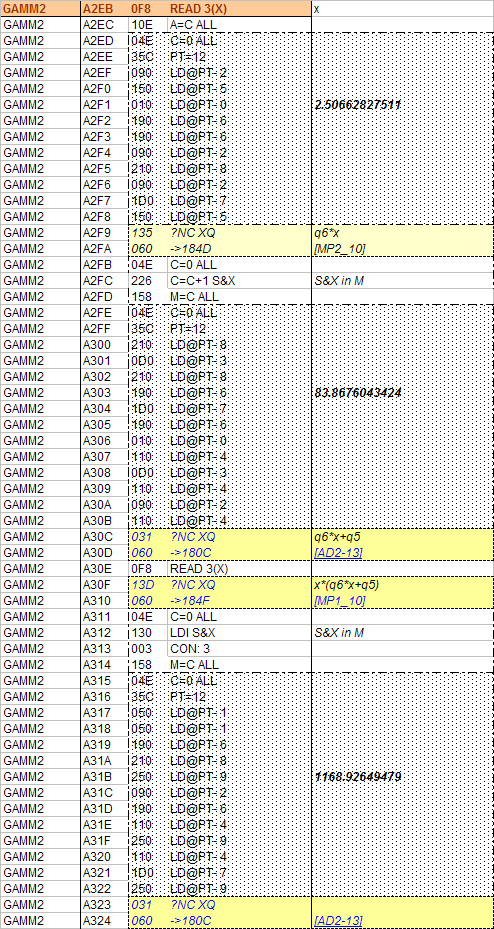
Putting it all together – Gamma for x>0 as a 13-digit function.[]
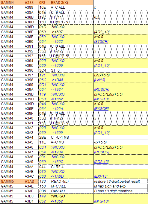
Just to go with a bang, here’s an example that consolidates many of the tips & tricks seen before. We’ll now write a routine to calculate the Gamma function of positive real numbers. We’ll use the Lanczos approximation with 12-digit coefficients, as follows:
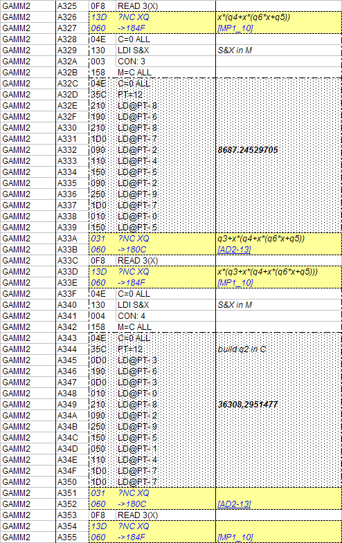
q0 = 75122.6331530
q1 = 80916.6278952
q2 = 36308.2951477
q3 = 8687.24529705
q4 = 1168.92649479
q5 = 83.8676043424
q6 = 2.5066282
Our function should give exact integer results for the natural numbers, since it’s wellknown that G(x) = (x-1)!. And here’s the source code for such a feat:
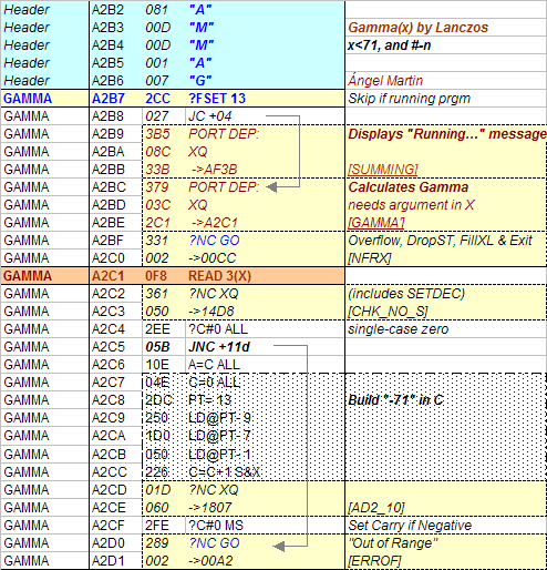
The function uses a subroutine because gamma is also used in the Bessel functions code – implemented all in MCODE in the SandMath Module for integer and real orders, but as they say, that’s another story…
We start by making sure we’ll be within the 41 numeric range. Since we know that factorials for numbers greater than 69 will exceed it, we impose the restriction that x must be less than 71. Nevertheless there’s also a final overflow check at the very end. Then we take on the product loop as seen in example #9 before. Note the handy utilization of the scratch registers routines, as well as the “fake” upgrade of x to a 13digit form for convenience sake.
Note also that we save the partial result in the scratch registers for later use. Next comes the long but simple polynomial term, written using Honer’s method to take advantage of its efficiency. Also partially seen in example #10, here’s where we use registers C&M for the coefficients, as second operands for the multiplication. This is done to use all digits up, for extended precision in the calculations.
At the end of this we’ll divide the partial result by the result from the productory loop, using the scratch registers again.
Yes this is long, but stick around a little longer, the best is yet to come… (after all programming is not always such an exciting ride).
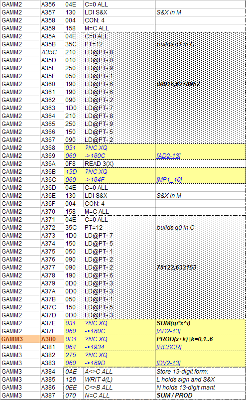
Lastly it comes the more involved phase, where we’ve used registers N and 4(L) as temporary scratch as well, since Q & “+” are already taken. Note that we’re using the exponential form of the power expression for simplicity:
(x+5,5)^(x+0.5)* exp[-(x+5.5)] = exp[ (x+0,5)*Ln(x+5.5) – (x+5.5)]
That’s all folks; hope this journey through the archeological SW department has been interesting to you all.